6 Sampling and Coverage
Where this chapter fits. Step 5 of the research process is to plan the sample. This chapter covers whom to ask and how to select them.
6.1 An Accurate Total and an Uneven Count
The 2020 Census counted 331.4 million people. Two years later, the Census Bureau reported how accurate the count had been. For the nation as a whole, the result was good. The estimated net error for people living in households was 0.24 percent, an undercount of about 782,000 people. That figure was within the range that chance alone could produce.
The national figure combined errors in both directions. The bureau estimated that the census missed 18.8 million people. It also counted millions of people twice or in the wrong place, and it filled in records for households that did not respond. The misses and the extra counts nearly canceled out in the total.
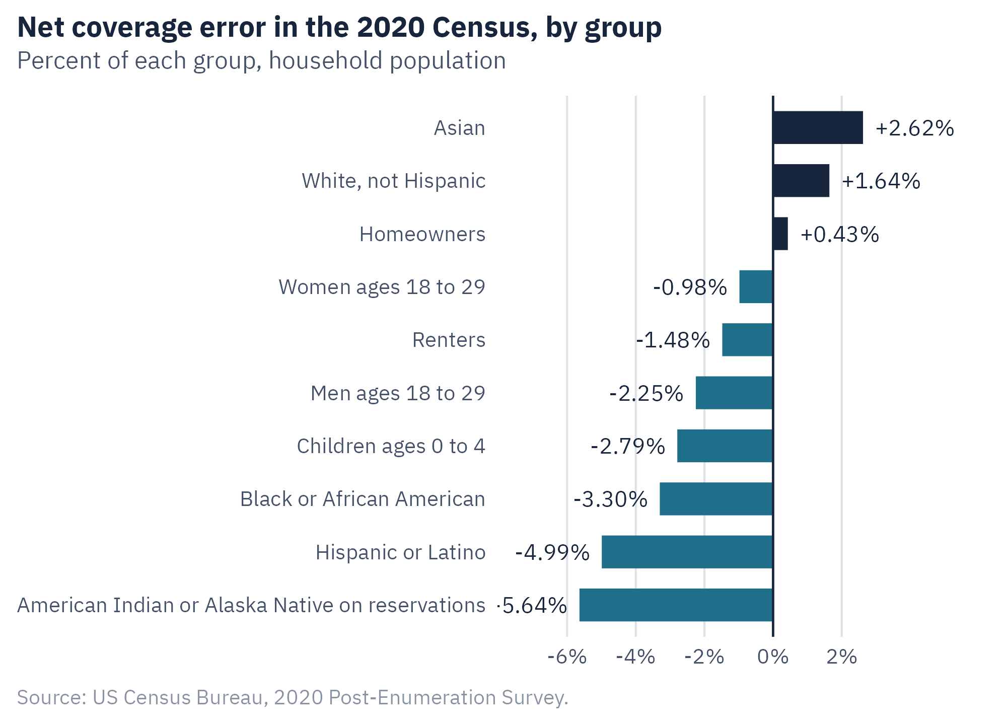
They did not cancel out for every group. Figure 6.1 shows the net error for several groups.
The census undercounted Hispanic residents by 4.99 percent and Black residents by 3.30 percent. It undercounted American Indians and Alaska Natives living on reservations by 5.64 percent. It undercounted children under age 5 by 2.79 percent and renters by 1.48 percent. It overcounted non-Hispanic white residents by 1.64 percent, Asian residents by 2.62 percent, and homeowners by 0.43 percent.
Census counts decide how seats in Congress are divided among the states. They also guide the distribution of federal funds. A group that is undercounted receives less of both.
The census tries to count everyone and still misses people at different rates. A survey, which contacts only a sample, faces the same problem at every step. This chapter covers how samples are drawn, how much a sample result can vary, and how a sample can leave people out.
6.2 Population, Frame, and Sample
Three terms from Chapter 2 organize this chapter.
The target population is the group the study aims to describe. The sampling frame is the list from which the sample is drawn. The sample is the set of units selected from the frame.
A census attempts to collect data from every unit in the population. A sample survey collects data from part of it. A census is not always more accurate than a sample. A census of a large population needs a very large field staff, and errors in the field are hard to control at that scale. A well-run sample can spend more effort on each case. The Census Bureau measures the accuracy of the census with a sample survey.
6.3 Probability Sampling
In a probability sample, every unit in the frame has a known chance of selection that is greater than zero. Chance decides which units are selected. This property allows the researcher to calculate how much the result could vary from sample to sample.
Four designs are common.
Simple random sampling. Every unit has the same chance of selection, and every possible sample of a given size is equally likely. It is the simplest design to analyze. It requires a complete list of the population, which is often not available.
Systematic sampling. The researcher picks a random starting point and then selects every kth unit on the list. To draw 100 from a list of 5,000, select every 50th name. The method is easy to carry out. It works well unless the list has a repeating pattern that matches the interval.
Stratified sampling. The researcher divides the population into groups, called strata, and draws a random sample within each one. A county survey could stratify by district so that every district is represented. A researcher can also sample a small group at a higher rate so that it has enough cases to analyze. Weights then restore each group to its true share.
Cluster sampling. The researcher selects groups of units and then surveys units within the selected groups. A national survey may select counties, then blocks within those counties, then households within those blocks. This is multistage sampling. It lowers the cost of travel and does not need a list of every person in the country. People in the same cluster tend to be alike. A cluster sample is therefore less precise than a simple random sample of the same size.
Table 6.1 compares the four.
| Design | How units are selected | Main advantage | Main limit |
|---|---|---|---|
| Simple random | Every unit has an equal chance | Simple to analyze | Needs a complete list |
| Systematic | Every kth unit after a random start | Easy to carry out | Patterns in the list can bias it |
| Stratified | Random samples within groups | Each group is represented | Needs group membership before sampling |
| Cluster | Random groups, then units within them | Lower cost, no full list needed | Less precise for the same sample size |
6.4 Samples Without Known Chances
In a nonprobability sample, the chance that a unit is selected is unknown. Three kinds are common.
A convenience sample takes whoever is easy to reach, such as shoppers at one store or students in one class. A quota sample recruits until it has a set number of people in each category, such as 50 men and 50 women. A snowball sample asks each participant to refer others. It is used to reach groups that have no list, such as people who use a particular drug.
Most online surveys today use opt-in panels. People sign up to take surveys for payment, and researchers draw from the panel. The panel is a nonprobability sample, because people chose to join. Panel companies use quotas and weights to make the sample resemble the population on age, sex, race, and education. The sample can match the population on those variables and still differ on the variable being studied.
Nonprobability samples have uses. They suit pilot tests, experiments with random assignment, and studies of groups that cannot be listed. They do not support a margin of error, because the theory behind it assumes that chance decided who was selected.
The best-known failure of a large nonprobability sample is from 1936. The Literary Digest magazine mailed about 10 million ballots before the presidential election and received about 2.4 million back. It drew its mailing list largely from telephone directories and automobile registrations. The poll predicted that Alf Landon would win with 57 percent of the vote. Franklin Roosevelt won with about 61 percent. The frame left out many voters with lower incomes, and the people who returned ballots differed from those who did not. A sample of 2.4 million did not correct for either problem.
6.5 How Much a Sample Can Vary
A probability sample supports a statement about sampling error. For a proportion from a simple random sample, the margin of error at the 95 percent level is calculated as follows.
\[\text{margin of error} = 1.96 \times \sqrt{\frac{p(1-p)}{n}}\]
In the formula, \(p\) is the sample proportion and \(n\) is the sample size. Suppose a survey of 400 adults finds that 30 percent rent their homes.
- Multiply \(p\) by \(1 - p\). The result is \(0.30 \times 0.70 = 0.21\).
- Divide by \(n\). The result is \(0.21 / 400 = 0.000525\).
- Take the square root. The result is \(0.0229\).
- Multiply by 1.96. The margin of error is \(0.045\), or 4.5 percentage points.
The survey’s estimate is 30 percent, plus or minus 4.5 points. If the survey were repeated many times, about 95 percent of such intervals would contain the true proportion.
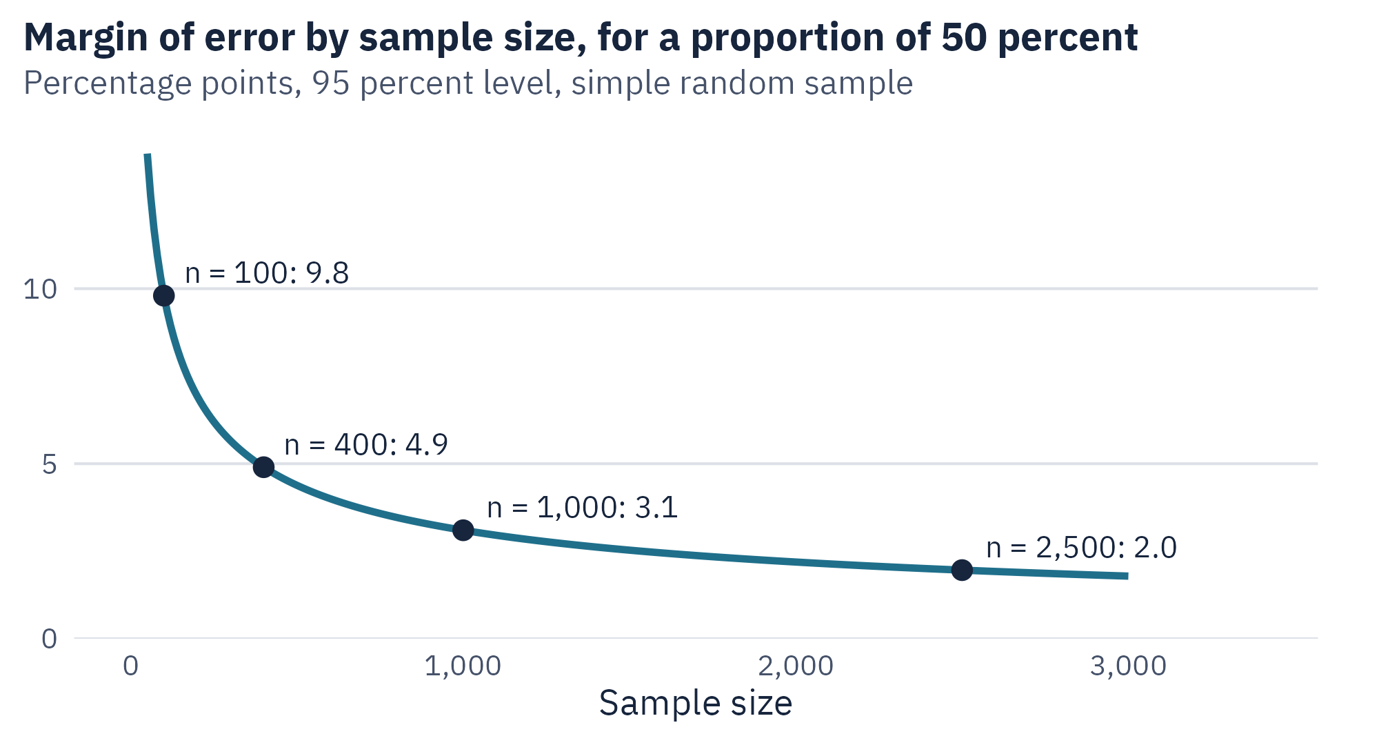
Figure 6.2 shows two facts about sample size.
First, the gain from each added case shrinks. Going from 100 to 400 cases cuts the margin from 9.8 points to 4.9. Going from 1,000 to 2,500 cuts it from 3.1 to 2.0. To cut the margin in half, the sample has to be four times as large.
Secondly, the size of the population does not appear in the formula. A sample of 1,000 gives about the same margin for a city of 200,000 as for a country of 300 million. A sample is more precise when it has more units. It does not depend on what share of the population they represent, unless that share is large.
Subgroups Have Their Own Sample Sizes
A survey of 1,000 people has a margin of about 3 points for the whole sample. If 120 of them are renters under age 30, the margin for that subgroup is about 9 points. Plan the sample size for the smallest group you intend to report.
6.6 Coverage and Nonresponse
The margin of error describes sampling error only. Two other sources often matter more.
Coverage. A frame can leave out part of the population. The census builds its frame from a master list of addresses. Some homes are harder to list. Examples are a household in a converted garage, a family doubled up in one apartment, and a rural home with no street address. The undercount of renters, young children, and residents of reservations follows from where the frame is weakest.
Nonresponse. A unit can be on the frame, be selected, and still not respond. The response rate is the share of selected units that complete the survey. A low response rate does not by itself bias the result. Bias arises when the people who respond differ from those who do not on the variable being measured. In the census, households that did not respond were visited by field staff. When that failed, the bureau used information from neighbors or from administrative records, or it filled in the record with a statistical estimate.
Researchers adjust for both problems with weights. If young adults are 20 percent of the population and 10 percent of the respondents, each young respondent is counted twice. Weighting corrects the sample on the variables used to build the weights. It does not correct a difference on a variable that the weights did not include.
6.7 Work With the Data: Sampling Explorer
This chapter has described two different problems. A sample varies from one draw to the next, and a frame can leave people out. The tool shows both in one simulated population of 10,000 households. The true share with a housing cost problem is 23.8 percent.
Open Sampling Explorer in its own window
- Leave the sample size at 400 and the share of renters missing at 0 percent. Press “Draw 300 samples.” Read the middle 95 percent of the estimates.
- Raise the sample size and draw again. The estimates move closer together. Their average stays near 23.8 percent.
- Set the share of renters missing from the frame to 40 percent. Draw again. Read the average and the bias.
- With renters still missing, raise the sample size once more and draw.
In the last step the estimates move closer together around the wrong value. With 40 percent of renters missing, the average is about 21 percent and the bias is close to 3 points at any sample size. A larger sample reduces variable error. It does not repair a frame that leaves people out.
6.8 How the Census Checks Itself
The Census Bureau estimates its own error with a method called dual-system estimation. Biologists use the same idea to estimate the size of a wildlife population, and they call it capture and recapture.
After the 2020 Census, the bureau carried out a separate survey of about 10,000 census blocks. Interviewers listed every household in those blocks independently of the census. The bureau then matched the survey records to the census records, person by person.
The logic uses three numbers. Suppose that in one area the census counted 900 people. The independent survey found 800 people. Of those 800, 720 could be matched to a census record.
- Calculate the share of survey people the census found. The share is \(720 / 800 = 0.90\).
- Treat that share as the census coverage rate for the area. The census found about 90 percent of the people.
- Divide the census count by the coverage rate. The estimate of the true population is \(900 / 0.90 = 1{,}000\).
- Compare with the census count. The census missed about 100 people, an undercount of 10 percent.
The bureau applies this logic within groups defined by age, race, and housing tenure. The results are the estimates in Figure 6.1. The survey is itself a sample, and so each estimate has its own sampling error.
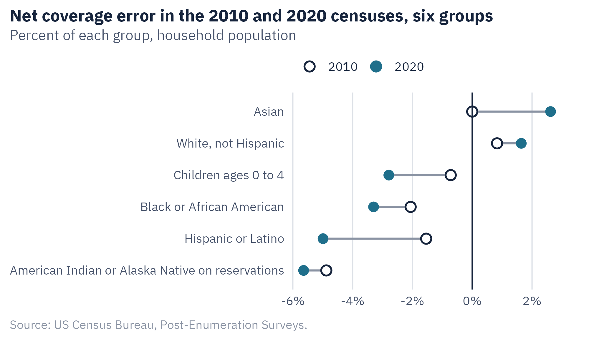
Figure 6.3 compares 2020 with 2010. The undercount of Hispanic residents rose from 1.54 percent to 4.99 percent. The undercount of children under 5 rose from 0.72 percent to 2.79 percent. The 2020 Census was conducted during a pandemic, which disrupted field work. The national total remained accurate, and the errors for groups grew.
Ethics Moment: Who Bears the Cost of a Weak Frame
Coverage error does not fall evenly. The people a frame misses are more often renters, young children, people of color, and people in rural areas. When a survey guides how money or services are distributed, those groups receive less. A researcher can reduce the harm in three ways. Spend more of the budget on the groups that are hardest to reach. Report results for those groups with their own margins of error. State plainly who the frame could not reach.
AI Reality Check: Synthetic Respondents Are Not a Sample
Some companies now offer “synthetic respondents.” A language model is asked to answer survey questions as if it were a person with a given age, income, and location. The answers are fast and cheap. They are not a sample of any population. The model produces the answers that its training data make likely for that description. It cannot report an opinion that formed last month, and it tends to produce answers that vary less than those of real people. Synthetic answers can help test whether a questionnaire works. They should not be reported as the views of a population.
6.9 Putting It All Together
A probability sample gives every unit in the frame a known chance of selection. Simple random, systematic, stratified, and cluster designs are the main types. A probability sample supports a margin of error, which depends on the sample size and not on the size of the population. Nonprobability samples, including opt-in online panels, do not support a margin of error.
The margin of error covers sampling error only. Coverage error arises when the frame leaves out part of the population. Nonresponse error arises when those who respond differ from those who do not. Weights can correct for differences on the variables they include.
The 2020 Census shows how errors can cancel in a total and remain large for groups. The national net error was 0.24 percent. The undercount was 4.99 percent for Hispanic residents and 5.64 percent for American Indians and Alaska Natives living on reservations.
6.10 Looking Ahead
Once a sample is drawn and a questionnaire is ready, data collection begins. Chapter 7 covers what happens between the first response and a clean data file. The case is an online panel in which some of the responses did not come from attentive people.
6.11 Further Reading and References
- US Census Bureau (2022). Census Bureau Releases Estimates of Undercount and Overcount in the 2020 Census (Release CB22-CN.02). The source for the coverage estimates in this chapter.
- Khubba, S., Heim, K., and Hong, J. (2022). National Census Coverage Estimates for People in the United States by Demographic Characteristics. US Census Bureau. The technical report on the Post-Enumeration Survey.
- Cohn, D., and Passel, J. S. (2022). Key Facts About the Quality of the 2020 Census. Pew Research Center. A summary of omissions, duplicates, and filled-in records.
- Lohr, S. L. (2021). Sampling: Design and Analysis (3rd ed.). CRC Press. A full textbook on sampling designs.
- Squire, P. (1988). Why the 1936 Literary Digest poll failed. Public Opinion Quarterly, 52(1), 125 to 133.
- Mercer, A., Lau, A., and Kennedy, C. (2018). For Weighting Online Opt-In Samples, What Matters Most? Pew Research Center.
6.12 Key Terms
- Census. An attempt to collect data from every unit in a population.
- Cluster sampling. Selecting groups of units and then surveying units within them.
- Convenience sample. A sample of whoever is easy to reach.
- Dual-system estimation. Estimating coverage by matching two independent counts of the same area.
- Margin of error. The amount a sample result is expected to vary because of sampling, at a stated level of confidence.
- Multistage sampling. Cluster sampling carried out in more than one step.
- Nonprobability sample. A sample in which the chance of selection is unknown.
- Opt-in panel. A group of people who signed up to take surveys.
- Probability sample. A sample in which every unit in the frame has a known chance of selection above zero.
- Quota sample. A sample recruited until each category has a set number of people.
- Response rate. The share of selected units that complete the survey.
- Simple random sampling. A design in which every unit has an equal chance of selection.
- Snowball sample. A sample built by asking participants to refer others.
- Stratified sampling. Drawing random samples within groups of the population.
- Systematic sampling. Selecting every kth unit after a random start.
- Weights. Numbers that make some respondents count more or less so the sample matches the population.
6.13 Exercises
Check Your Understanding
- State the difference between a probability sample and a nonprobability sample. Which one supports a margin of error?
- The 2020 Census had a net error of 0.24 percent and missed 18.8 million people. Explain how both statements can be true.
- Why does a sample of 1,000 give about the same margin of error for a city as for a country?
- A survey has a response rate of 9 percent. Under what condition would its results still be unbiased?
Apply It
- A survey of 900 adults finds that 42 percent have a regular doctor. Calculate the margin of error at the 95 percent level. Show each step.
- A census counts 4,500 people in an area. An independent survey finds 1,000 people there, and 920 of them match a census record. Estimate the true population and the percent undercount. Show each step.
- A county has 60,000 adults in the city and 20,000 in rural areas. You can afford 800 interviews and want a margin of about 5 points for each area. Propose a stratified design and explain how you would weight the results.
Think Deeper
- The census overcounted homeowners and undercounted renters. List three features of renting that could explain the difference. Which source of error from Chapter 2 does each one involve?
- An online panel is weighted to match the population on age, sex, race, and education. A client says it is “representative.” What would you want to know before you agreed?
- Use the file
ch06-census-coverage.csv. A state receives $2,000 per resident each year from programs tied to census counts. Estimate what a 4.99 percent undercount costs a community of 50,000 Hispanic residents over ten years. State what your estimate assumes.