8 The Analysis Plan and the Report
Where this chapter fits. Step 7 of the research process ends with analysis and interpretation, and step 8 is the report. This chapter covers how to plan the analysis before seeing the data and what a report has to contain.
8.1 One File, Several Answers
In May 1985, the Census Bureau’s monthly household survey asked workers about their pay. Economists have used a sample of 534 of those workers as a teaching dataset for decades. The file records each worker’s pay, sex, years of education, years of work experience, occupation, union membership, and a few other characteristics. Pay is expressed as an annual figure, calculated from the hourly wage at 2,000 hours a year.
The file contains 245 women and 289 men. Suppose an analyst is asked one question. How large was the pay gap between women and men?
The file supports several answers.
- Women’s mean pay was $15,758 and men’s was $19,990. By this measure, women earned 79 cents for each dollar men earned.
- Women’s median pay was $13,600 and men’s was $17,860. By this measure, the figure is 76 cents.
- Among workers with the same education and experience, women earned about 22.7 percent less than men.
- Among workers with the same education, experience, occupation, union status, and region, women earned about 19.3 percent less.
Each figure is calculated correctly. Each one answers a slightly different question. An analyst who runs all of them and reports one has made a choice that the reader cannot see.
This chapter covers the last two steps of a study. The first is the analysis plan, which is written before the data are examined. The second is the report, which tells readers what was done.
The file is from 1985. It is used here to show how analysis choices affect a result. It does not describe pay today.
8.2 Write the Plan First
An analysis plan states how the data will be analyzed. It is written before the analyst looks at the results. A plan answers five questions.
- What is the outcome? Name the variable and how it is measured. Here it is annual pay.
- What is the comparison? Name the groups or the relationship of interest. Here it is women compared with men.
- What statistic will summarize it? State whether the plan uses a mean, a median, a ratio, or a model.
- What will be held constant? List any variables the analysis will adjust for, with the reason for each.
- Which cases are included? State any rules for excluding cases, as described in Chapter 7.
The plan connects the analysis to the research question from Chapter 1. A different question leads to a different plan. “How much less do women earn than men?” calls for a comparison with no adjustment. “Are women paid less than men for the same work?” calls for an adjustment for the kind of work. Neither question is the correct one. They are different questions, and a report should say which one it answers.
8.3 Choosing a Summary
The first choice is the statistic.
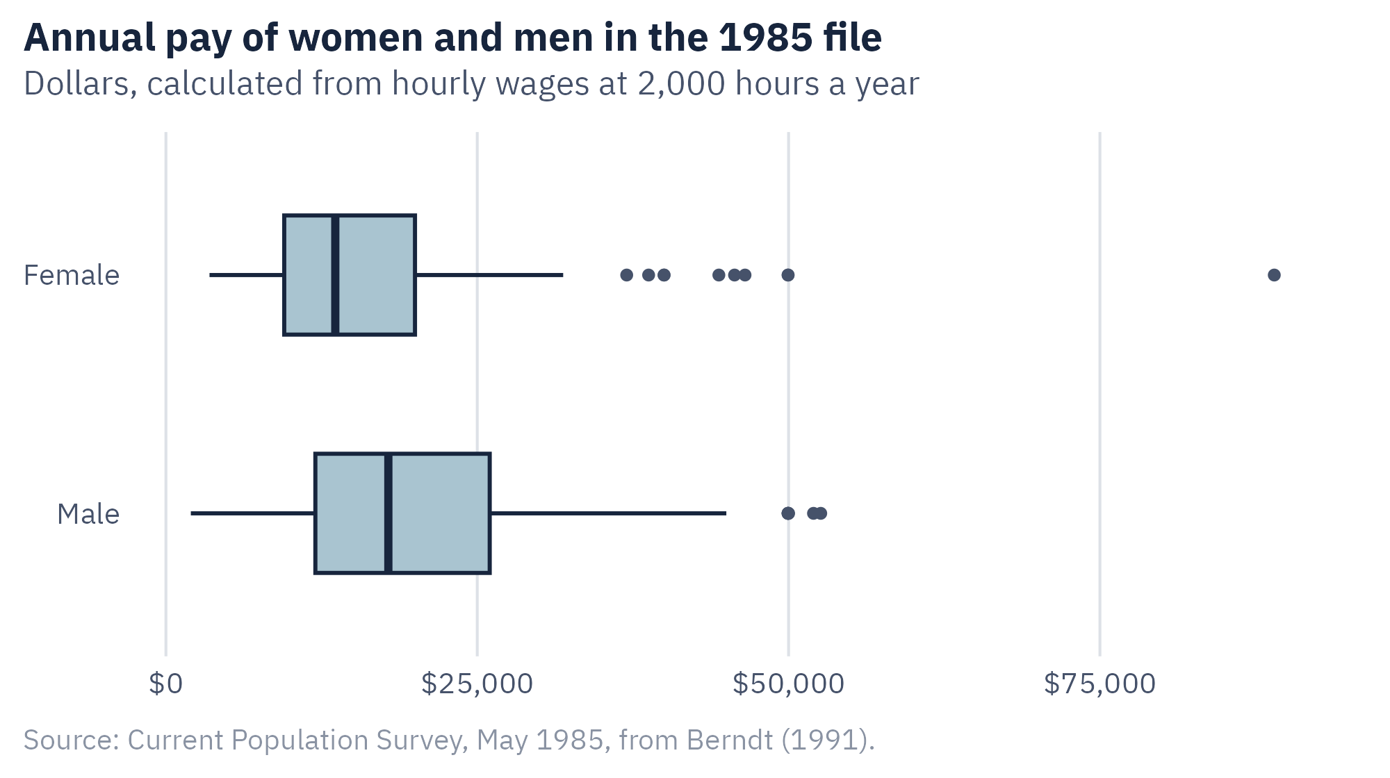
Figure 8.1 shows that pay is skewed. Most workers are grouped at the lower end, and a few earn far more. The highest value in the file is $89,000, which is more than five times the median.
In a skewed distribution, the mean is pulled toward the long tail. The median is not. For pay, income, and wealth, the median usually describes the typical case better than the mean. A plan should state which one it will use and should not switch after the results are known.
The second choice is how to express the gap. The same two medians can be reported in three ways.
- As a difference, women earned $4,260 less.
- As a ratio, women earned 76 cents for each dollar.
- As a percent difference, women earned 24 percent less.
The three statements describe one fact. The ratio and the percent difference can be compared across years, because they do not depend on the price level. The dollar difference is easier for a general reader to picture. A report can give more than one form, and it should label each one.
8.4 What “Adjusted” Means
Women and men in the file differ in more than pay. They work in different occupations, and men are more likely to belong to a union. An analyst may want to compare women and men who are alike in these respects.
A regression model does this. It estimates how the outcome changes with one variable while the other variables in the model are held constant. Chapter 11 of Margin of Error covers the method. For this chapter, one idea is enough. A variable that the model holds constant is a control variable, and the gap that remains is the adjusted gap.
Figure 8.2 shows the gap under four sets of control variables.
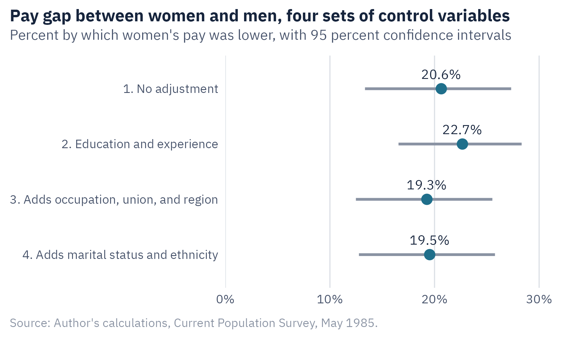
With no adjustment, women earned 20.6 percent less. When the model holds education and experience constant, the gap is 22.7 percent. The gap grows because the women in this file had the same average education as the men and slightly more experience. Those two variables do not account for any of the gap.
When the model also holds occupation, union membership, and region constant, the gap falls to 19.3 percent. Part of the raw gap is associated with the kinds of jobs women and men held. Adding marital status and ethnicity changes the estimate very little.
8.5 A Control Variable Is a Choice About the Question
It can seem that more control variables always give a better answer. They give an answer to a narrower question.
Consider occupation. In the file, 76 of the 245 women worked in office jobs, and 126 of the 289 men worked in manual jobs. Holding occupation constant compares women and men within the same type of job. That comparison is useful if the question is whether an employer pays women and men differently for the same work.
Suppose, though, that women were steered away from higher-paying occupations. Then occupation is one of the routes by which sex affects pay. A model that holds occupation constant removes that route from the estimate. The adjusted gap will be smaller, and the part that was removed is a result of the process being studied.
A variable that lies on the path between a cause and an outcome is a mediator. Adjusting for a mediator answers the question “What remains of the gap after this path is set aside?” That can be the right question. The analyst has to choose it on purpose and say so.
For this reason, a careful report gives both figures. The unadjusted gap describes the overall difference in pay. The adjusted gap describes the difference among workers who are alike on the listed variables. A reader needs both, with the list of control variables, to understand either.
8.6 Work With the Data: Pay Gap Explorer
The last two sections showed that the adjusted gap depends on which variables are held constant. The tool lets you make that choice yourself for the 534 workers in the 1985 file.
Open Pay Gap Explorer in its own window
- Read the gap with no adjustment. Women’s hourly pay was lower by 20.6 percent.
- Select education and experience. Read the new gap and its confidence interval.
- Add occupation. The gap falls. Decide whether occupation is a fair variable to hold constant, or a route by which pay comes to differ.
- Look at the small marks. Each is the gap under one of the 64 possible sets of control variables. Find the smallest and the largest.
- Select all six variables and read the gap.
With all six variables held constant, the gap is 19.5 percent. Every one of the 64 choices is defensible, and they do not agree. An analyst who chooses the set after seeing the results can report almost any figure in that range. This is the reason to write the plan first.
The file is ch08-wage-gap.csv at quant.marginoferrormedia.com/data.
Three Checks on a Control Variable
Before you add a control variable, ask three questions. Could it affect both the group and the outcome? If so, it is a confounder, and adjusting for it is appropriate. Could the group affect it? If so, it may be a mediator, and adjusting for it changes the question. Is it measured well? A poorly measured control adjusts only partly.
8.7 Many Reasonable Analyses
The four estimates in Figure 8.2 do not exhaust the choices. An analyst could also use the mean or the median, or include or exclude part-time workers. The analyst could group occupations in a different way or drop the highest earners. Each choice is defensible. Together they produce dozens of possible analyses.
Gelman and Loken (2014) call this the garden of forking paths. Few analysts set out to mislead. The more common problem is that an analyst makes each choice after seeing how it affects the result. The analyst then settles on the path that gives the expected answer.
A well-known study measured how much the path matters. Silberzahn and colleagues (2018) gave one dataset and one research question to 29 teams of analysts. The question was whether soccer referees gave more red cards to players with darker skin. The teams used 21 different sets of control variables. Twenty teams found a statistically significant effect, and nine did not. The estimated effects ranged from slightly negative to nearly three times the odds.
Two practices reduce the problem.
Preregistration. The analyst records the analysis plan in a public, time-stamped registry before analyzing the data. Readers can then compare the report with the plan. Analyses that were not in the plan can still be reported, and they are labeled as exploratory.
Reporting several specifications. The analyst runs every reasonable version of the analysis and reports all of the results, as in Figure 8.2. If the estimates agree, the finding does not depend on one choice. If they disagree, the reader learns that it does.
8.8 Stating Uncertainty
The 534 workers are a sample. A different sample would give somewhat different estimates. The lines in Figure 8.2 are confidence intervals. Each one shows a range of values that are consistent with the data at the 95 percent level.
For the model with education and experience, the interval runs from about 17 to about 28 percent. A report should give the interval with the estimate. “Women earned about 23 percent less, with a 95 percent confidence interval of 17 to 28 percent” is a complete statement. “Women earned 22.7 percent less” suggests more precision than a sample of 534 can support.
The interval covers sampling error only. As Chapter 2 explained, it does not cover errors in how pay was reported or in who responded to the survey.
Two rules of presentation follow.
- Round to the precision the data support. With an interval that is about 12 points wide, a decimal place adds nothing. Report “about 23 percent.”
- Do not treat overlapping estimates as different. The four intervals in Figure 8.2 overlap. The data do not show that the four specifications give different answers.
8.9 What a Report Has to Contain
A report allows a reader to judge the result and another researcher to repeat the study. The American Association for Public Opinion Research lists the items that a survey report should disclose. Table 8.1 adapts that list and links each item to a chapter of this book.
| Item to report | What to state | Chapter |
|---|---|---|
| Research question | The population, the concept, and the time and place | 1 |
| Definitions | How each construct was defined and measured | 1 and 4 |
| Design | Whether the study was a survey, an experiment, or another design | 3 |
| Question wording | The exact wording and order of the questions reported | 5 |
| Sample | The frame, the sampling method, and the sample size | 6 |
| Dates and mode | When and how the data were collected | 7 |
| Response and exclusions | The response rate, or a statement that none applies, and every exclusion rule with counts | 6 and 7 |
| Weights | Whether weights were used and what they were based on | 6 |
| Analysis | The statistic, the control variables, and whether the plan was registered | 8 |
| Uncertainty | The margin of error or confidence interval, and what it leaves out | 2 and 8 |
| Limitations | Who was left out and what the design cannot show | All |
| Sponsor | Who paid for the study and who conducted it | 5 |
A limitations section is not an apology. It tells the reader where the result applies. For the 1985 file, three limits matter. The data are four decades old. The sample is 534 workers from one month. The file has no measure of hours worked per week, job tenure with the current employer, or the size of the firm.
The order of a report also matters. Most readers want the finding first. A common structure is a one-paragraph summary, the main findings with figures, the methods, and the limitations. Technical detail goes in an appendix. Make It Visible, the visualization book in this series, covers how to design the figures.
Ethics Moment: The Number That Gets Repeated
A report on a pay gap will be quoted by people on different sides of a debate. One side may quote the unadjusted gap as evidence of unequal pay for equal work, which it does not measure. The other side may quote the adjusted gap as evidence that no problem exists, which it does not show either. An analyst cannot control how a number is used. The analyst can make misuse harder. Put both figures in the same sentence. State what each one measures. Do not publish either figure without the other.
AI Reality Check: A Model Will Run Any Analysis You Ask For
A language model with access to a data file can run all four specifications in this chapter in under a minute. It can run forty more. This makes the forking paths problem worse, because each added analysis costs nothing. A model will also write a confident paragraph about whichever result you ask it to describe. Use the tool for what it does well, which is running a plan you have already written. Write the plan first. Ask the model to carry it out and to report every specification. Then check a sample of its numbers against your own calculation.
8.10 Putting It All Together
An analysis plan is written before the results are seen. It names the outcome, the comparison, the statistic, the control variables, and the cases included. Each of these choices can change the answer.
In the 1985 file, women earned between about 19 and 23 percent less than men, depending on the control variables. The unadjusted gap describes the overall difference. The adjusted gap describes the difference among workers who are alike on the listed variables. A control variable that lies on the path from cause to outcome changes the question being answered.
Many reasonable analyses of one dataset can give different results. Preregistration and reporting several specifications make the choices visible. A report states the estimate with its uncertainty, lists every item a reader needs to judge it, and describes its limits.
8.11 Looking Back and Looking Ahead
This book has followed one path. A question became a definition and then a measure. The measure was built into a tested questionnaire. A sample was drawn, data were collected and cleaned, and the analysis was planned and reported. At each step, a choice affected the final number.
Numbers answer questions of how many and how much. They are less able to answer why people act as they do or what an experience was like for them. Those questions call for a different kind of data. Beyond the Numbers, the companion to this book, covers research based on interviews, focus groups, and written text.
8.12 Further Reading and References
- Berndt, E. R. (1991). The Practice of Econometrics: Classic and Contemporary. Addison-Wesley. The source of the 534-worker file from the May 1985 Current Population Survey.
- Gelman, A., and Loken, E. (2014). The statistical crisis in science. American Scientist, 102(6), 460 to 465. The source of the phrase “garden of forking paths.”
- Silberzahn, R., Uhlmann, E. L., Martin, D. P., and others (2018). Many analysts, one data set: Making transparent how variations in analytic choices affect results. Advances in Methods and Practices in Psychological Science, 1(3), 337 to 356.
- Blau, F. D., and Kahn, L. M. (2017). The gender wage gap: Extent, trends, and explanations. Journal of Economic Literature, 55(3), 789 to 865. A review of research on adjusted and unadjusted gaps.
- Nosek, B. A., Ebersole, C. R., DeHaven, A. C., and Mellor, D. T. (2018). The preregistration revolution. Proceedings of the National Academy of Sciences, 115(11), 2600 to 2606.
- American Association for Public Opinion Research. Code of Professional Ethics and Practices and Transparency Initiative Disclosure Elements. The disclosure standards adapted in this chapter.
8.13 Key Terms
- Adjusted gap. A difference between groups that remains after a model holds other variables constant.
- Analysis plan. A statement, written before the results are seen, of how the data will be analyzed.
- Confidence interval. A range of values consistent with the data at a stated level of confidence.
- Control variable. A variable that a model holds constant.
- Garden of forking paths. The many reasonable analyses that one dataset allows.
- Limitations. A statement of who was left out and what the design cannot show.
- Mediator. A variable on the path between a cause and an outcome.
- Preregistration. Recording an analysis plan in a public registry before analyzing the data.
- Regression model. A method that estimates how an outcome changes with one variable while others are held constant.
8.14 Exercises
Check Your Understanding
- List the five questions an analysis plan answers.
- Why does the median usually describe typical pay better than the mean?
- Explain the difference between a confounder and a mediator. Why does it matter which one a control variable is?
- What does a 95 percent confidence interval cover, and what does it leave out?
Apply It
- In a company, women’s median pay is $58,000 and men’s is $66,000. Express the gap as a difference, a ratio, and a percent difference. Show each calculation.
- Use the file
ch08-wage-gap.csv. Calculate the median pay of women and men who are union members and of those who are not. Describe the result in two sentences. - Write an analysis plan for this question. “Do renters in the county report worse health than homeowners?” Answer all five questions and name two control variables with a reason for each.
Think Deeper
- A report states, “After controlling for occupation, hours, and industry, the pay gap is 5 percent.” What question does that figure answer? What question does it leave open?
- In the red card study, 29 teams reached different results from one dataset. Does this mean the question cannot be answered? What should a reader conclude from the full set of results?
- Choose a published survey report. Check it against Table 8.1. Which items does it disclose, and which are missing? What does the missing information prevent you from judging?